CindyGL Tutorial - Textures (with Live Coding)
In this tutorial, you will learn how to read from textures or the webcam. Then you will also learn how to write to textures, and we will build an application that uses a feedback loop for an efficient rendering procedure.
Prerequisites
In this tutorial, we assume that you have already seen how to create basic fundamental CindyJS applets that use colorplot.
Loading a texture to CindyJS
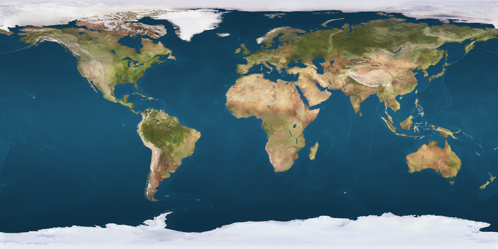
When you are creating an HTML applet, then you can load images. First, put a picture you want to load to CindyJS in a folder. For this tutorial, we will use the free texture earth.jpg (from http://planetpixelemporium.com/earth.html). If you want to create an applet that loads the image, which has to be stored in the same folder where you want to create your applet, you can copy&paste the following code and save loadimage.html:
<!DOCTYPE html>
<html>
  <head>
    <script type="text/javascript" src="https://cindyjs.org/dist/latest/Cindy.js"></script>
    <title>Loading Images in CindyJS</title>
  </head>

  <body>
    <div id="CSCanvas"></div>

    <script id="csdraw" type="text/x-cindyscript">
      drawimage(A, B, "earth");
    </script>

    <script type="text/javascript">
    CindyJS({
      scripts: "cs*",
      geometry: [
        {name:"A", kind:"P", type:"Free", pos:[-9, -8]},
        {name:"B", kind:"P", type:"Free", pos:[9, -9]},
      ],
      ports: [{
        id: "CSCanvas",
        width: 500,
        height: 300,
      }],
      images: {"earth": "earth.jpg"}
    });
    </script>
  </body>
</html>
If you open the HTML-file you will see this applet:
The important part of this source is the configuration images: {"earth": "earth.jpg"}, which loads the local image that can be accessed via the string "earth". The command drawimage(A, B, "earth"); draws the picture on the canvas by pinning the lower left and lower right corner to the position of the points A and B.
Live-Coding within this tutorial
You can also do some live coding within this tutorial. The editable code on the right is used as draw-script. By clicking on the large yellow boxes with CindyScript code the code is automatically copied to the applet on the right. You can assume that the applet on the right has earth.jpg loaded in "earth". The drawing-area covers all all coordinates between $-1.2$ and $1.2$.
For example, you can make the image dance if you use this code:
drawimage((-1,sin(seconds())), (1,cos(seconds())), "earth");Reading at a given pixel-coordinate
Instead of accessing the whole picture via drawimage, its colors at a given pixel-coordinate can be read of with the imagergb-function.
If one talks about a certain pixel-coordinate, one needs to specify a coordinate system. The function imagergb(‹pos›,‹pos›,‹imagename›,‹pos›) returns the color of the at the coordinate given as the fourth argument while assuming that the lower left and right corner coincide with the first two arguments respectively. The result is encoded as a 3-component vector with each entry ranging from 0 to 1, representing the RGB-value. You can think of pinning the given image on the drawing canvas and accessing the color from that pinned image the given canvas coordinates.
The following code reads the color underneath the mouse position:
drawimage((-1,-1), (1,-1), "earth");
rgb = imagergb((-1,-1), (1,-1), "earth", mouse());
draw(mouse(), color->rgb, size->30);
drawtext(mouse(), rgb, color->[1,1,1]);
Also if one wants to access images within colorplot, there is no way avoiding imagergb.
A colorplot that reads the colors pixel by pixel from the image can emulate a drawimage command:
colorplot(
  imagergb((-1,-1), (1,-1), "earth", #) // '#' iterates over all possible pixel values
);
This it looks a bit different than
drawimage((-1,-1), (1,-1), "earth");because imagergb returns the color black ([0,0,0]) whenever a coordinate outside the image is accessed. If the program within colorplot evaluates to a four component vector, then the fourth component is interpreted as an alpha-value between $0$ and $1$ where $0$ means invisible and $1$ opaque. CindyJS provides the function imagergba, which will read a four-component vector including its alpha-value. Pixels outside the image will have alpha value $0$. Hence the following script produces the same image as drawimage:
colorplot(
  imagergba((-1,-1), (1,-1), "earth", #)
);
But we can do way more than mimicking drawimage. For example, we can read textures in way more individual way:
colorplot(
  imagergba((-1,-1), (1,sin(seconds())/2), "earth",
  #+0.04*(sin(40*#.x), cos(40*#.y)))
);
The additional term +0.3*(sin(4*#.x), cos(4*#.y)) distorts the image.
An often useful modifier for the imagergb-command is repeat->true. When a color outside the actual image is read, this modifier will take care that the image is interpreted as it was repeated again and again in both directions:
colorplot(
  imagergb((-1,-1), (1,-1), "earth", #*exp(1+sin(seconds())), repeat->true)
)
Beside playing with the input coordinates, you can also operate on the color space. For example, you can apply a sepia-filter on the image to make it look vintage:
colorplot(
  rgb = imagergb((-1,-1), (1,-1), "earth", #);
  brightness = rgb*[0.3, 0.6, 0.1]; // dot product
  brightness*[1.2,1,0.8] //scalar times vector
);
Mapping a texture to a sphere
Our aim is to map this map of the earth onto a sphere:
How can such a three-dimensional image of the earth obtained via a colorplot? You can consider this as a primer in ray-marching with colorplot. Let us imagine that behind each pixel with coordinate # is a ray. This ray will or will not intersect the sphere. If the ray eventually intersects the sphere, we compute the first intersection point between ray and sphere. Then, we apply a time-dependent rotation to the intersection point on the sphere and calculate the sphere-coordinate of the rotated point. We can determine which piece of earth lays at that sphere-coordinate by looking it up in the texture earth.jpg we will display the corresponding color at position #.
For mathematical simplicity, we will think of the earth as a unit sphere, which is the set of all points $$S^2 = \{ s \in \mathbb{R}^3 \mid s_1^2 + s_2^2 + s_3^2=1 \}.$$
Furthermore, let us agree on the convention that in three-dimensional space the $x$- and $y$-axes lie flat, while the $z$-axis points to the top. The $z$-axis will intersect both the north- and south-pole of our earth.
To make things easy, we will use the orthographic projection. So by the definition of our axes, we imagine that the ray
$$r_{\text{#}}(t) = (\text{#}.x, t, \text{#}.y)$$
lays behind a pixel with coordinates #.
Where does this ray $r_{\text{#}}$ intersect the unit sphere $S^2$ first? It is clear that it will intersect the unit-sphere if and only if $|\text{#}|<1$. Any intersection point s must fulfill $s_1^2 + s_2^2 + s_3^2=1$. The solution is s = (#.x, -re(sqrt(1-#*#)), #.y). The product #*# is an abbreviation for the dot-product of $\text{#}$ with itself and is equivalent to $x^2+y^2$ if $\text{#}=(x,y)$. The given s lays on the sphere because it fulfills
$$s_1^2+s_2^2+s_3^2 = x^2 + (1-(x^2+y^2)) + y^2 = 1.$$
We took the negative sign in the second component -re(sqrt(1-#*#)) to obtain the first intersection of the ray with the sphere. Let us start with the following toy-code:
colorplot(
  if(|#|<1,
    s = (#.x, -re(sqrt(1-#*#)), #.y); //point on S^2 "behind" pixel
    grey(s*[0,-1,1]) //scalar product of normal and some random vector
    ,
    red(1) //use red if no sphere-intersection
  )
);
Let us compute the coordinates of s on the sphere using inverse trigonometric functions with lon = arctan2([s.x, s.y]); and lat = re(arcsin(s.z));. We obtain angles $lon\in (-\pi, \pi)$ and $lat\in (-\tfrac{\pi}{2}, \tfrac{\pi}{2})$. We want to read of the pixel from our texture earth.jpg, which is an equirectangular projection of our earth. In order to read the correct coordinates, we pin the lower left and lower right corner to $(-\pi, -\tfrac{\pi}{2})$ and $(\pi, -\tfrac{\pi}{2})$ respectively. In CindyScript this means, we take the color with imagergb((-pi, (-pi/2)), (pi, (-pi/2)), "earth", (lon, lat)).
Altogether, we now have:
colorplot(
  if(|#|<1,
    s = (#.x, -re(sqrt(1-#*#)), #.y); //point on S^2 "behind" pixel
    lon = arctan2([s.x, s.y]);
    lat = re(arcsin(s.z));
    imagergb((-pi, (-pi/2)), (pi, (-pi/2)), "earth", (lon, lat))
    ,
    red(1) //use red if no sphere-intersection
  )
);
Now let us make the applet look a bit nicer than this! Obviously, this red background is unaesthetic. Do we rather want to have a black background? This can be done by replacing red(1) with red(0) or [0,0,0].
To make everything more interesting and simulate the sunlight, we also compute a light-factor light = (max(0.1, s*[-.3,-1,0.1])); based on the dot product between the normal-vector s and the randomly chosen sun-direction [-.3,-1,0.1]. If we multiply our color output with this factor, we get some shading:
colorplot( if(|#|<1,
  s = (#.x, -re(sqrt(1-#*#)), #.y);
  light = (max(0.1, s*[-.3,-1,0.1]));
  lon = arctan2([s.x, s.y]);
  lat = re(arcsin(s.z));
  imagergb((-pi, (-pi/2)), (pi, (-pi/2)), "earth", (lon, lat))*light;
  , [0,0,0]
));
What about some animation? Let us rotate s around the z-axis to obtain another point on the sphere, which later will determine the colors of the pixels. The rotation around the z-axis can be done with a rotation matrix. Matrices are natively supported within CindyJS:
colorplot( if(|#|<1,
  s = (#.x, -re(sqrt(1-#*#)), #.y);
  light = (max(0.1, s*[-.3,-1,0.1]));
  s = [[cos(seconds()), sin(seconds()), 0],
       [-sin(seconds()), cos(seconds()), 0],
       [0,0,1]]*s; //matrix*vector
  lon = arctan2([s.x, s.y]);
  lat = re(arcsin(s.z));
  imagergb((-pi, (-pi/2)), (pi, (-pi/2)), "earth", (lon, lat))*light;
  , [0,0,0]
));
The direction of the rotation was chosen such that the sun will rise in the east.
Altogether, if you would like to create this spinning earth as an HTML-Applet you could have the following source:
<!DOCTYPE html>
<html>
  <head>
    <script type="text/javascript" src="https://cindyjs.org/dist/snapshot/Cindy.js"></script>
    <title>A spinning earth</title>
  </head>

  <body>
    <div id="CSCanvas"></div>
    <script id="csdraw" type="text/x-cindyscript">
      R = [
        [cos(seconds()), sin(seconds()), 0],
        [-sin(seconds()), cos(seconds()), 0],
        [0,0,1]
      ];

      colorplot(
        if(|#|<1,
          s = (#.x, -re(sqrt(1-#*#)), #.y); //point on S^2 "behind" pixel
          light = (max(0.1, s*[-.3,-1,0.1]));
          s = R*s;
          lon = arctan2([s.x, s.y]);
          lat = re(arcsin(s.z));
          light*imagergb((-pi, (-pi/2)), (pi, (-pi/2)), "earth", (lon, lat));
          ,
          [0,0,0]
        );
      )
    </script>

    <script type="text/javascript">
    CindyJS({
      scripts: "cs*",
      autoplay: true,
      ports: [{
        id: "CSCanvas",
        width: 500,
        height: 500,
        transform: [{
          visibleRect: [-1.2, 1.2, 1.2, -1.2]
        }]
      }],
      images: {"earth": "earth.jpg"}
    });
    </script>
  </body>
</html>
Accessing the Webcam
If you want to use a camera, you have to evoke video = cameravideo(); once. Usually, this is done in the init-script. If you have a webcam, and you want to play around with it in live-coding, please click here to evoke video = cameravideo(); in the live-coding app and accept to access your webcam, otherwise the code snippets in this section will not work. Several browsers indicate that the webcam is active in their address bar.
Now if you apply the code
drawimage((-1,0), (1,-1), video);you should see your webcam video-stream.
If you read the stream video within colorplot through imagergb, you can mess up yourself however you like. You can deform yourself:
colorplot(
  imagergb((-1,-.5),(1,-.5), video, #*|#|);
);
Or you can operate on the color space and show yourself in inverted colors:
colorplot(
    [1,1,1]-imagergb((-1,0),(1,0), video, #, repeat->true);
);
Can you map yourself on the spinning earth above?
It is also possible to load videos to a CindyJS applet by adding an option videos: {"video": "videoname.mp4"}. Then after running playvideo("video"), you can access the image in the same way. If you want to see an example, there is a CindyJS applet deforming a video shot by Henry Segerman with a spherical camera.
Writing to Textures
colorplot can, instead of drawing to the whole drawing screen, plot to a texture.
One can create a texture with createimage(‹imagename›,‹int›,‹int›) as described in the reference manual of CindyScript.
Then the texture is accessible via colorplot(‹pos›,‹pos›,‹imagename›,‹expr›) where the two first arguments specify the coordinates of the lower left and lower right point again. ‹imagename› is the target texture, and ‹expr› is the program that is executed for each pixel of the target texture depending on the pixel coordinate #.
In this live coding applet, a texture has automatically created in the initialization ('init') script via createimage("plot", 800, 800).
We can write something on this texture and output it as follows:
A = (-1,-0.5);
B = (.2,-1);
colorplot(A, B, "plot", //renders to "plot"
  grey(.5 + .5*sin(20*(#*#)))
);
drawimage(A, B, "plot");
You can change the coordinates A and B. However you always should see the section of essentially the same plot, because colorplot(A, B, ...) and drawimage(A, B, ...) have the same coordinate-system.
Both the commands colorplot and imagergb can be used with only a texture as an argument. Then CindyGL tries to fit the texture with the entire visible drawing area and uses the coordinates of this environment.
Feedback-loops
If one reads and writes to the same texture with some deformations in between, we can simulate a video feedback loop, where one points a camera to a screen that displays the image that the camera records:
offset = 0.02*(cos(seconds()), sin(seconds()));
factor = 0.9+.05*sin(seconds());
colorplot("plot", // plots to texture "plot"
  // read old texture and make it a little bit brighter!
  imagergb("plot", (#-offset)/factor) + (4,2,3)/100
);
colorplot(imagergba("plot", #)); //output "plot"
Note that pixels outside the image "plot" are interpreted as black.
Try to replace the offset with the current mouse position! Can you simulate a rotated camera that points to a screen?
A little miracle occurs when a complex transformation is applied before reading the pixel-coordinate:
c = -0.32-0.14*i+.02*sin(seconds());
colorplot("plot",
 z = complex(#*1.5);
 if(|z|<2, // if |z|<2 take the color at z^2+c
  imagergb("plot", z^2+c) + (1,2,3)/100,
  (0, 0, 0) // otherwise: output black.
 )
);
colorplot(imagergba("plot", #));
That applet is inspired by Felix Woitzel. We see the Julia set! Try to replace c = -0.32-0.14*i+.02*sin(seconds()); with c = complex(mouse()); to obtain some interactivity.
Every point on the screen is represented through a complex number $z_0 \in \mathbb{C}$,
The feedback loop computes the escape time for the sequence $z_{n+1} = z_n^2+c$ for every pixel simultaneously.
A more sophisticated version of this applet can be found in our gallery. Also, Limit sets of IFS and Kleinian Groups can be rendered in CindyGL utilizing this technique.
You can continue the tutorial on GPGPU computations through CindyGL.