CindyGL Tutorial - GPGPU through color plots

In this tutorial, we want to build an applet that simulates a reaction-diffusion equation on the GPU. As a primer, we will first simulate Conway's Game of Life on the GPU. The trick in all these applications is to store the data on textures. Using colorplot, one can write to a texture; And by using imagergb, one can read from a texture.

Prerequisites

We assume that you already have seen how one can create texture-feedback loops in CindyGL and you know how to create your CindyJS-applets.

Conway's Game of Life

Conway's Game of Life is an example of a cellular automaton. Think of a large grid/square lattice of cells that are either living or dead. In this grid, each cell has eight neighbors that determine its new state. If a living cell

has fewer than two living neighbors it dies because of underpopulation,
has two or three living neighbors it will continue to live,
has more than three living neighbors it dies because of overpopulation.

A dead cell can become a living one if it has exactly three live neighbors. All these transitions take place at the same time. We will build an applet gol.html, which simulates the cellular automaton on the GPU:

(if this applet got stuck in an uninteresting pattern, then reload the page to restart the simulation)

We want to simulate this automaton via colorplot on the GPU. It is reasonable that we can use a texture that represents the state of the cells through the colors of each pixel (which conveniently also lay in such a grid).

If you want to program along, you can start with boilerplate.html and modify it while reading this tutorial.

Suppose, we want to "play" the game of life on a 128x128 texture (powers of two are always good because textures with this dimensions fix nicely in the texture-buffer; However other dimensions should work as well). So let us create in the init-script a 128x128 texture via

createimage("gol", 128, 128);

Now, if we want to access the cell, which is in column x and row y (from the bottom), we could use imagergb((0,0), (128,0), "gol", (x,y), interpolate->false). We need the modifier interpolate->false, because otherwise the pixel (1,1) would be interpreted as the average of the four pixels $(0,0), (0,1), (1,0), (1,1)$, which have their centers at $(0.5, 0.5), (0.5, 1.5), (1.5, 0.5), (1.5, 1.5)$:

pixel coordinates

With interpolate->false the function imagergb returns the color of the pixel that is closest to the given coordinate. To solve the issue one could offset everything with $(0.5,0.5)$. But it is more convenient to use interpolate->false which rounds any coordinate down to the closest pixel center. So our call imagergb((0,0), (128,0), "gol", (x,y), interpolate->false) remains readable and gives the desired answers and en passant also increases the performance of the simulation.

The code imagergb((0,0), (128,0), "gol", (x,y), interpolate->false) can be simplified to imagergb("gol", (x,y), interpolate->false) if we specify that the global drawing domain just has the same domain. This can be done by adding the option

transform: [{
  visibleRect: [0, 128, 128, 0]
}]

to the CindyJS-initialization function.

Thus let us define a helper function

get(x, y) :=  imagergb("gol", (x,y), interpolate->false, repeat->true).r;

that returns only the red-value of the corresponding pixel. This number, which will either be $0$ or $1$, will be the state of the cell $(x,y)$.

In order to initialize the texture "gol", we will initialize it some random states via

colorplot("gol", if(random()>.6,1,0)); //random values as starting image

random() is a function that returns, independently for every pixel, a random value between $0$ and $1$. So with $60%$- probability a pixel gets color $1$, otherwise $0$. Color $1$? You may wonder that $1$ is a number, and not a 3-component RGB color vector. CindyGL will interpret a number number as output-variable automatically as gray(number)=[number, number, number].

Now let us proceed with to the draw-script: For each pixel # we need to count the number of neighbors and then color the pixel accordingly.

We will overwrite the old texture "gol" with a new texture via

colorplot("gol", newstate(#.x, #.y)); //overwrite texture "gol"

where newstate(x, y) is defined as follows:

newstate(x, y) := (
  number = countneighbors(x, y); //number of living neighbors
  if(get(x, y) == 1,

    //if the cell lives then it will die if it has less than 2 neighbours or more than 3 neighbours
    if((number < 2) % (number > 3), 0, 1),

    //if cell was dead then 3 living neighbours are required to be born
    if(number == 3, 1, 0)
  )
);

That essentially implements the rules from above where 1 stands for living and 0 for dead.

Only the function countneighbors is missing. It should go through all 8 (Moore)-neighbour-cells of (x, y) and count those neighbours (nx, ny) that have get(nx, ny)==1. One could write here the sum of 8 terms or one could use two nested repeat, loops. CindyJS also has list-operations that (maybe) simplify this:

deltas = [(-1,-1), (-1,0), (-1,+1), (0,-1),  (0,+1), (+1,-1), (+1,0), (+1,+1)];
countneighbors(x, y) := sum( apply(deltas, delta, get(delta.x + x, delta.y + y)

apply converts the list of deltas in a list of get-values that are either 0 or 1. sum computes the sum of all those values.

The function newstate should be evaluated to overwrite in the draw-script. So we put:

<script id="csdraw" type="text/x-cindyscript">
  colorplot("gol", newstate(#.x, #.y)); //overwrite texture "gol"

We also want to output the image. One could use drawimage( (0,0), (0, 128), "gol"), which however looks blurry, because drawimage uses interpolation for its output. To avoid this function, we can use a colorplot that simply uses our get-function:

  colorplot( get(#.x, #.y) );

Altogether we have the following source:

<!DOCTYPE html>
<html>
  <head>
    <script type="text/javascript" src="https://cindyjs.org/dist/latest/Cindy.js"></script>
    <script type="text/javascript" src="https://cindyjs.org/dist/latest/CindyGL.js"></script>
    <title>Conway's Game of Life in CindyGL</title>
  </head>

  <body>
    <div id="CSCanvas"></div>

    <script id="csinit" type="text/x-cindyscript">
      createimage("gol", 128, 128);
      colorplot("gol", if(random()>.6,1,0)); //random values as starting image

      get(x, y) :=  imagergb("gol", (x,y), interpolate->false, repeat->true).r; //Tourus world

      deltas = [(-1,-1), (-1,0), (-1,+1), (0,-1),  (0,+1), (+1,-1), (+1,0), (+1,+1)];
      countneighbors(x, y) := sum( apply(deltas, delta, get(delta.x + x, delta.y + y)));

      newstate(x, y) := (
        number = countneighbors(x, y); //number of living neighbors
        if(get(x, y) == 1,

          //if the cell lives then it will die if it has less than 2 neighbours or more than 3 neighbours
          if((number < 2) % (number > 3), 0, 1),

          //if cell was dead then 3 are required to be born
          if(number == 3, 1, 0)
        )
      );
    </script>

    <script id="csdraw" type="text/x-cindyscript">
      colorplot("gol", newstate(#.x, #.y)); //overwrite texture "gol"
      colorplot( get(#.x, #.y) );
    </script>

    <script type="text/javascript">
    CindyJS({
      scripts: "cs*",
      autoplay: true,
      ports: [{
        id: "CSCanvas",
        width: 512,
        height: 512,
        transform: [{
          visibleRect: [0, 128, 128, 0]
        }]
      }]
    });
    </script>
  </body>
</html>

A CindyGL implementation of the Game of Life with a bit more interaction can be found here.

Numerical simulation of a reaction-diffusion equation

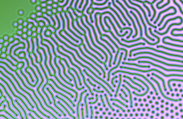
We want to create a simulation of a Reaction–diffusion system, more precisely of the Gray-Scott model. We will create a CindyJS-applet reactdiff.html, which generates patterns like this on the GPU:

screenshot of modified reactdiff.html

We start with gol.html and adopt the code until we have reactdiff.html, because it turns out that the computational schemes are very similar.

However, we need a higher resolution than we had for the Game of Life. To increase the resolution from 128 to 512 you can search and replace every 128 with a 512. Furthermore, we like to call our texture "state" instead of "gol", so let us perform another search&replace.

We want to simulate two chemicals and their interaction on the plane. Chemical one is steadily poured into the system while chemical two is removed from it (the feed-parameter f and kill-parameter k will regulate this behaviour). The chemicals diffuse, where the first chemical spreads twice as fast than the second one. Furthermore, one "portion" of the first and two portion the second chemical react to three portions of the second chemical.

Let us call the local densities of the two chemicals $q_1$ and $q_2$. More formally, there are two space and time dependent functions $q_1(x,y,t), q_2(x,y,t) \in [0,1]$ that give the density of chemicals. The described behaviour can be modelled through the following equation:

$$\partial q_1= \nabla^{2}q_1 - q_1 q_2^2 + f\cdot (1-q_1)$$

and

$$\partial q_2= \tfrac{1}{2} \nabla^{2} q_2 + q_1 q_2^2 + (k+f)\cdot q_2$$

Karl Sims gives a good explanation for the Gray-Scott model on his website.

We will discretize this differential equation and simulate it on the GPU. There are two discretizations: in time and in space space. Firstly, space will be discretized to a grid and secondly time canonically to equally spaced time steps. Similar to the cellular automaton we have seen before, we will compute the new state out of the old state for each time step.

For this system, we need to store two parameters (instead of one dead/living-state) in the texture "state". Let us utilize the first two components of the RGB-color information (i.e. red and green) for that purpose! So let us rewrite the get-function (which, so far, only has read the red component) to

get(x, y) :=  (
  rgb = imagergb("state", (x,y), interpolate->false);
  (rgb.r, rgb.g) //return value
);

Furthermore, let us also introduce the (almost inverse) store function which converts a two-component vector q to a color, which then can be stored on the texture:

store(q) := (q_1, q_2, 0);

To initialize the state q for each pixel we will run the following function in the init-script:

initialimage(x) := store((0.2+.3*random(), .2+.2*random())); //random values as starting image
colorplot("state", initialimage(#));

Our newstate-function, which will is executed for each pixel in each rendering step, will now model the differential equations:

newstate(x, y) := (
  q = get(x,y);
  laplacian = computelaplacian(x, y);

  f = 0.02+0.06*y/512;   // feed rate - appropriately chosen
  k = 0.059+0.007*x/512; // kill rate - appropriately chosen

  deltaq = [laplacian_1 - q_1*q_2*q_2 + f * (1-q_1),
      0.5 * laplacian_2 + q_1*q_2*q_2 - (k+f) * q_2];

  store(q+deltaq)
);

To begin, we read the current state at the pixel and compute the 2-component discrete laplacian $\nabla q$ via a helper function. The feed and kill parameters f and k are set such that they vary over the plane. With this, we generate a mixture of various patterns: This helps us to solve the diplomatic problem of finding perfect parameters that suit well for everybody!

The 2-component vector deltaq contains the (discrete) derivatives given by the two equations above. With store(q+deltaq) it will be added to the current state q to approximate the next new state and stored in the texture (technically the color-vector will be returned). One could sample the time finer if one adds a factor as store(q+0.1*deltaq).

The discrete laplacian is computed via a convolution with the following kernel:

kernel = [[0.05, 0.2, 0.05],
           [0.2,   -1, 0.2],
           [0.05, 0.2, 0.05]];
computelaplacian(x, y) := (
  sum( apply(-1..1, dy,
      sum( apply(-1..1, dx,
          kernel_(dy+2)_(dx+2)*get(x+dx, y+dy)
      ))
    ))
);

The specific kernel was chosen, since it makes also the discrete Laplacian operator is rotation invariant.

We like that the states in "state" are updated through newstate in every draw-step. The draw-script is maximum evaluated 60 times in the second. That might be a bit too slow for us to see some fascinating movement. Therefore let us have ten updates for every draw step:

<script id="csdraw" type="text/x-cindyscript">    
  repeat(10, //do 10 steps of iteration in each drawing step
    colorplot("state", newstate(#.x, #.y)); //overwrite texture "state"
  );
  ...

If you have a really powerful graphic cards, this is the place, where you can benchmark it with having way more steps for each drawing iteration (and, of course, a higher resolution than 512x512)!

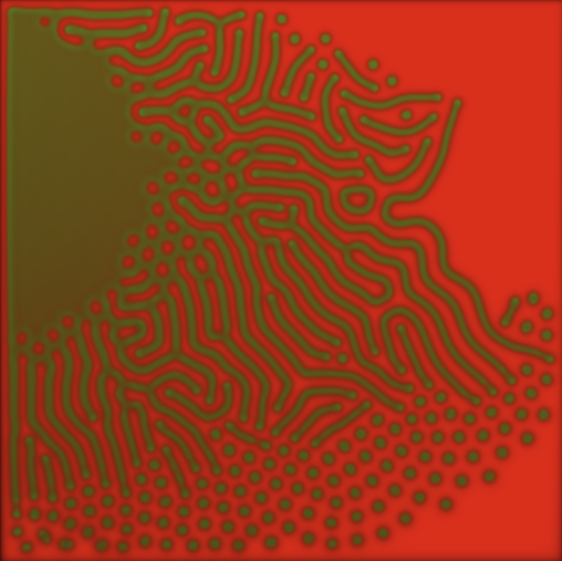
Now, finally we want to see the computed q-values, stored in "state" as output! If one uses drawimage((0,0),(512,0), "state"); then one would directly see what the texture stores:

texture "state" in reactdiff.html

Maybe you do not really like this colors. We can get a nicer colorization through a function that computes the output color after reading it from the texture:

//drawimage((0,0),(512,0), "state");
colorplot(
  q = get(#.x, #.y);
  0.7*hue(q_1)+[1,1,1]*(0.8-3*q_2)
)

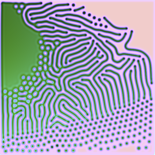
Here the first chemical determines the hue of the output color and the second chemical influences the brightness (the darker the higher the density of the second chemical): screenshot of reactdiff.html

If we run the applet now, we see how a "sponge" is growing from the area with a high feed-parameter spreading over the whole screen.

The applet reactdiff.html has the following source:

<!DOCTYPE html>
<html>
  <head>
    <script type="text/javascript" src="https://cindyjs.org/dist/latest/Cindy.js"></script>
    <script type="text/javascript" src="https://cindyjs.org/dist/latest/CindyGL.js"></script>
    <title>Reaction diffusion</title>
  </head>

  <body>
    <div id="CSCanvas"></div>

    <script id="csinit" type="text/x-cindyscript">
      createimage("state", 512, 512);

      get(x, y) :=  (
        rgb = imagergb("state", (x,y), interpolate->false);
        (rgb.r, rgb.g)
      );

      store(q) := (q_1, q_2, 0);

      initialimage(x) := store((0.2+.3*random(), .2+.2*random())); //random values as starting image
      colorplot("state", initialimage(#)); 

      kernel = [[0.05, 0.2, 0.05],
                 [0.2, -1, 0.2],
                 [0.05, 0.2, 0.05]];
      computelaplacian(x, y) := (
        sum( apply(-1..1, dy,
            sum( apply(-1..1, dx,
                kernel_(dy+2)_(dx+2)*get(x+dx, y+dy)
            ))
          ))
      );

      newstate(x, y) := (
        laplacian = computelaplacian(x, y);
        q = get(x,y);

        f = 0.02+0.06*y/512; //feed rate
        k = 0.059+0.007*x/512; //kill rate

        deltaq = [laplacian_1 - q_1*q_2*q_2 + f * (1-q_1),
                0.5 * laplacian_2 + q_1*q_2*q_2 - (k+f) * q_2];

        store(q+deltaq)
      );
    </script>

    <script id="csmousedown" type="text/x-cindyscript">
      errc(mouse());
      colorplot("state", store(min(1,|#-mouse()|/50)*get(#.x, #.y)));
    </script>

    <script id="csdraw" type="text/x-cindyscript">    
      repeat(10, //do 10 steps of iteration in each drawing step
        colorplot("state", newstate(#.x, #.y)); //overwrite texture "state"
      );
      //drawimage((0,0),(512,0), "state");
      colorplot(
        q = get(#.x, #.y);
        0.7*hue(q_1)+[1,1,1]*(0.8-3*q_2)
      )
    </script>

    <script type="text/javascript">
    CindyJS({
      scripts: "cs*",
      autoplay: true,
      ports: [{
        id: "CSCanvas",
        width: 512,
        height: 512,
        transform: [{
          visibleRect: [0, 512, 512, 0]
        }]
      }]
    });
    </script>
  </body>
</html>